Sampling Site

Figure 1. Site overview of the MSc research plot, labelled with the different vegetation growing on Stack 4 at Nutrien, Fort Saskatchewan, AB (augmented from (Nutrien Report, 2020)).
Part 1. Soil Core Experimental Design
|
Step 1

|
Step 2

|
Step 3

|
Step 4

|
Step 1: A total of 45 cores soil cores were taken from the study site seen in Figure 1., with 15 cores from areas consisting of poplar, willow, and grasses.
Step 2: Cores were stored in a freezer and before the core analysis it was sectioned by areas of interest and the length of each section was measured to obtain the volume. Sections changed if contents differed or when roots were gathered through noticeable cracks.
Step 3: The sections were based on categorical data such as the topsoil (TS), transition zone (TR), or PG categories: mixed PG and soil (MX); softly compacted PG (ST); medium compacted PG (MD); hard compacted PG (HD); clay (CL). Roots were gathered by s sifting sections through a 2.5mm sieve.
Step 4: Soil physical properties were done by measuring total weight and dry weight of the sections and included measures such as bulk density (Pb), gravimetric water content (θg), and volumetric water content (θv).
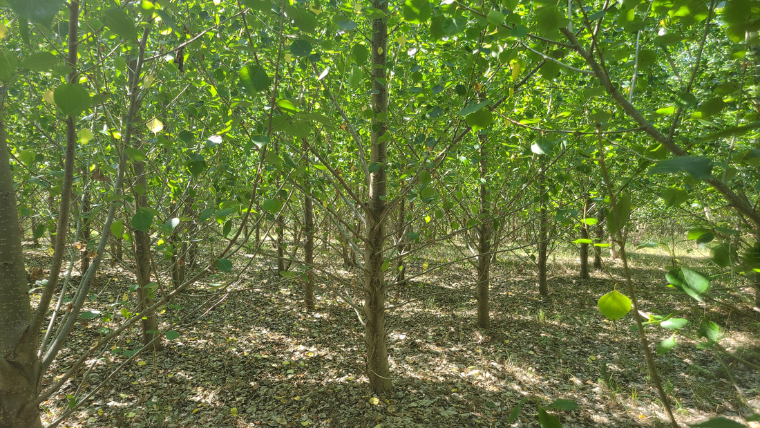
Poplar (Populus X ‘okanese’)
|

Willow (Salix Viminalis)
|
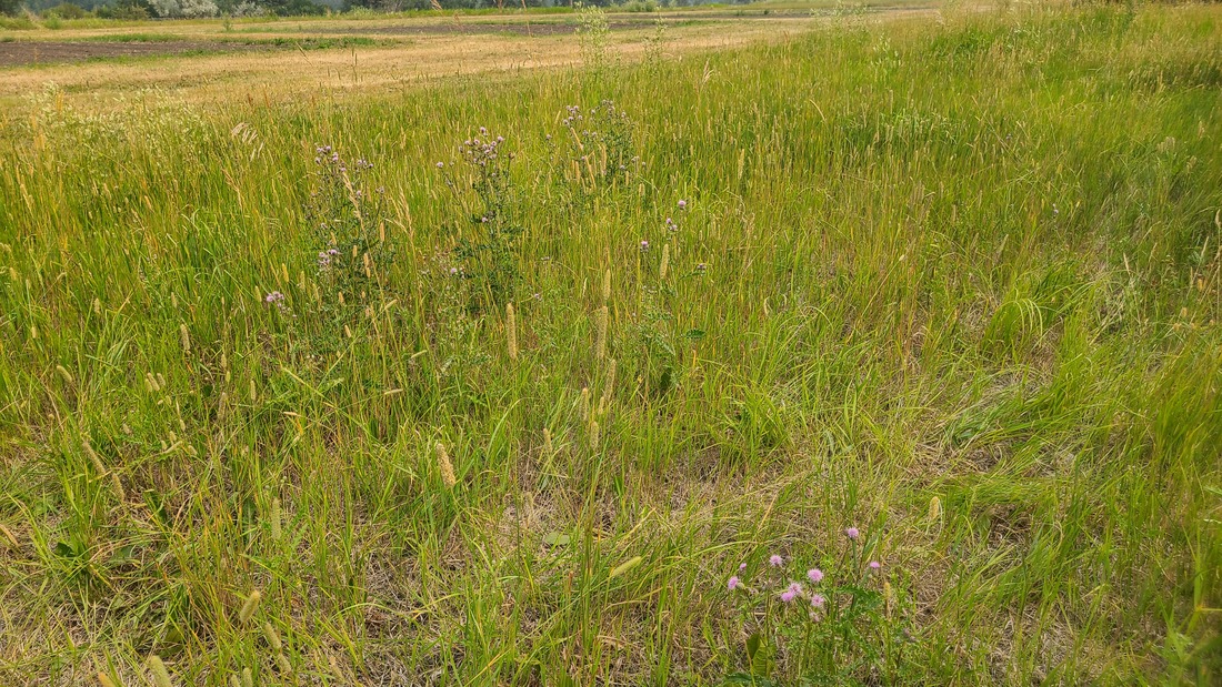
Grass (Spp.)
|
Part 2. Green House Experimental Design
|
Step 1

|
Step 2

|
Step 3

|
Step 4

|
Step 5

|
Step 1: Populus balsamnifera seeds collected from Alberta were seeded into plugs and grown for 6 weeks at 25°C, and 1000PAR in a greenhouse.
Step 2: Bulk densities (1.0 g/cm^3, 1.15 g/cm^3, 1.3 g/cm^3) were determined by taking the moisture content of each pot and calculating the weight needed to to get a dry weight within 9 inches of a 10 inch pot. The phosphogypsum was then compressed with a pneumatic press. A total of 60 pots, 10 for each replicate of the six treatments.
Step 3: A hole was drilled and the seedling, including the plug, were put into the compressed pots on July 27, 2022.
Step 4: Pots were brought up to specific water potentials (13.79 -kPa, 51.71 -kPa) and were watered everyday for 8 weeks to maintain the specific water potential. They were also fertilized each week with 20mL of 2g/L all purpose fertilizer solution.
Step 5: Plants were harvested on Sept 28, 2022 and above ground measurements were taken. Growth was determined by taking the difference between seedling height before planting and final heights. Both leaf area and caliper were taken and biomass for leaves and stems were combined into total above ground biomass.
Statistical Analysis Using R-Software
Part 1. Soil core Analysis
Sampling procedure on the reclaimed stack has limitations due to the quasi experimental design. Therefore, the statistical analysis can not include a comparison between the vegetation groups growing at the site. However, the question of whether there are relationships between soil physical factors and root density can be explored. To determine if there are any trends between root density and the physical properties measured in the core (bulk density, volumetric water content, and air filled porosity) I decided to use residual plots to determine the normality and scatter plots as my graphical exploration. To statistically determine if there were any significant correlations I used a one-way ANOVA. I then took all observations and did a linear regression analysis with a Holm-Bonferroni adjusted p-values to determine if there were any statistically significant results.
Part 2. Greenhouse experiment
The data exploration for this experiment consisted of Box and Whisker plots that were used to compare the different above ground measurements for all six treatments, and to clearly visualize the normality and variation within the replicates. The treatments were then put into a grouped bar chart with corresponding letter values using the R package multcompView to see the differences within and between treatments. I then used a multifactor ANOVA was to determine if there were any significant variations of total biomass(g), growth(cm), caliper(mm) and leaf are (cm2)between treatments of bulk density and water potential.
