Tables
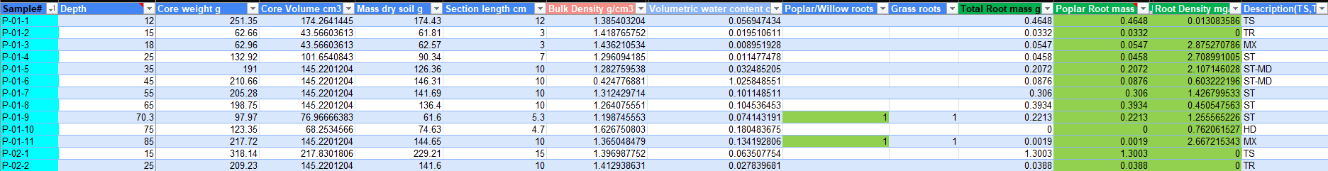
Table 1. Excel table representing the recorded and calculated measurements related to soil physical factors and root mass.
|
Design Variables: row.names- Unique ID, CORE.-Core sample number, SPP- Area where species is most present
Independent Variables: Discrete numerical: DEPTH- depth of core section (cm), BLKDN- Bulk Density (g/cm3), VWC-Volumetric water content (cm3H2O/cm3bulk soil), AIRFP- Air filled porosity (cm3air/cm3bulk soil), Factor Categorical: TYP-Description of core contents, the combination of bulk densities and water potential. Dependent Response Variables: Discrete Numerical: Root density (mg/cm3) |
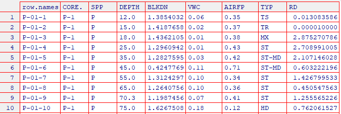
Table 2. R- Statistical data table showing the core data used in this analysis.
|
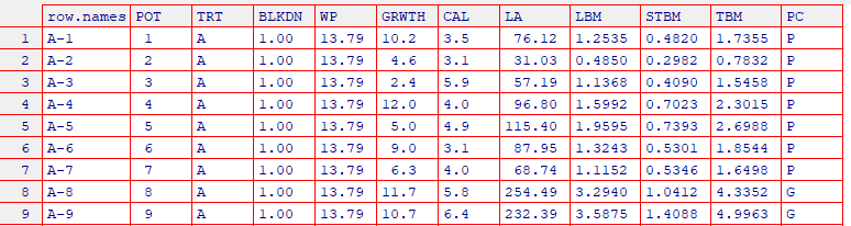
Table 3. Excel table representing the recorded above ground biomass data and measurements,

|
Design Variables: Pot- Individual identifier, row.names- Unique ID
Independent Variables: Discrete Numerical: BLKDN- Bulk Density (g/cm3), Water potential (-kPa), Factor Categorical: TRT- Treatment, the combination of bulk densities and water potential. Dependent Response Variables: Discrete Numerical: GRWTH- Growth measured from final measurement subtracted by the initial height of seedlings (cm), CAL- Caliper of the stem base width (mm), LA- Leaf Area (cm2), LBM- Total Leaf Biomass (g), STBM- Stem Biomass (g), TBM- Total Biomass (g), Factor Categorical: PC- Plant condition P-Poor, G-Good, E- Excellent |
Table 4. R- Statistical data table showing above ground measurements used in analysis.
|
Exploratory Graphics
Part 1. Soil Core Analysis
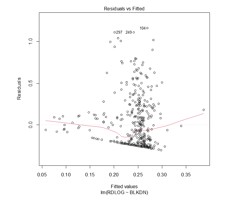
Figure 2. Residual plot of the log of root density (Log(Root density (mg/cm3)+1)) and BLKDN (bulk density g /cm3).
|
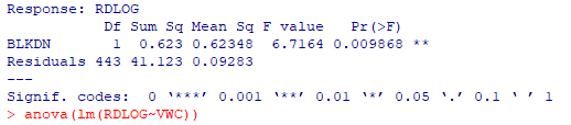
Table 3. Results computed from R-software showing a one-way ANOVA of (Log(Root density (mg/cm3)+1)) and BLKDN (bulk density g /cm3).
|
Interpretation
The above residual plot, Figure 2., shows that for the log of root density and bulk density is not normally distributed, but does seem to follow a trend. In Table 3., an ANOVA was preformed and shows that there is a significant p-value (<0.05), which signifies there is a significant relationship between root density and bulk density. |
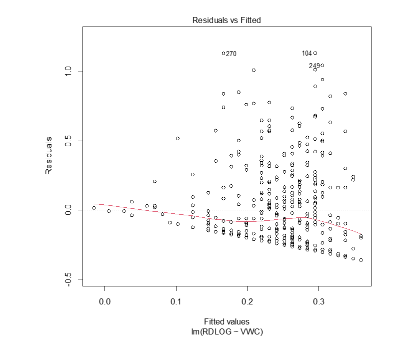
Figure 3. Residual plot of the log of root density (Log(Root density (mg/cm3)+1)) and VWC (volumetric water content (H20 (cm3)/ bulk soil (cm3)).
|
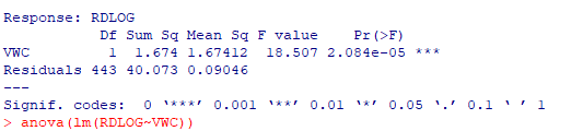
Table 4. Results computed from R-software showing a one-way ANOVA of (Log(Root density (mg/cm3)+1)) and VWC (volumetric water content (H20 (cm3)/ bulk soil (cm3)).
|
Interpretation
Figure 3. shows that for the log of root density and volumetric water content is not normally distributed data, but does seem to follow a trend similar to bulk density. In Table 4., an ANOVA was preformed and gave a highly significant p-value (<0.05), which means that there is a high likelihood of a relationship between root density and water content/availability. |
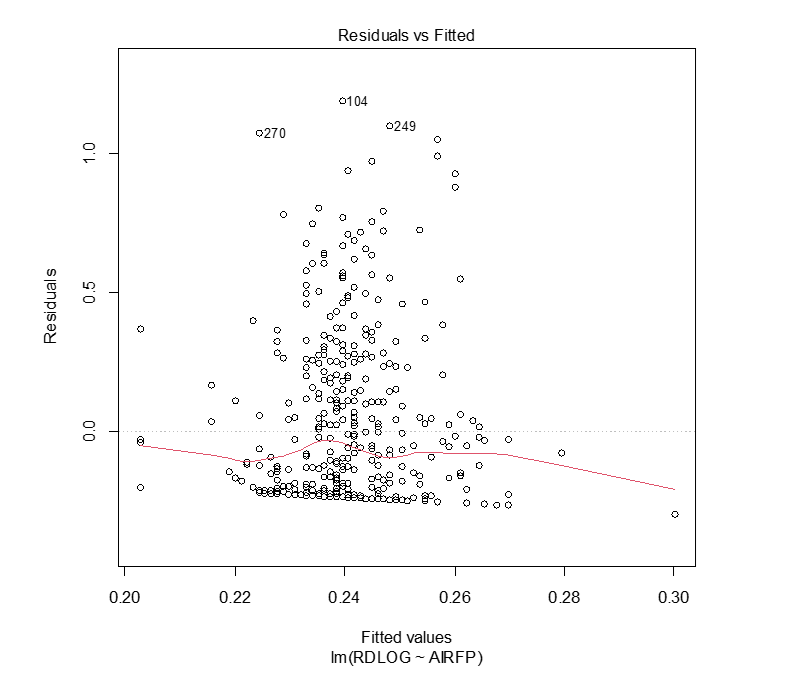
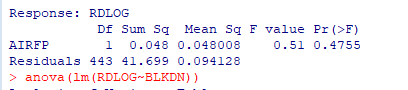
Figure 4. Residual plot of the log of root density (Log(Root density (mg/cm3)+1)) and AIRFP (Air-filled Porosity (air (cm3)/ bulk soil (cm3)).
|
Table 5. Results computed from R-software showing a one-way ANOVA of (Log(Root density (mg/cm3)+1)) and AIRFP (volumetric water content (air (cm3)/ bulk soil (cm3)).
|
Interpretation
In Figure 4. the log of root density and air filled porosity is not normally distributed data, which is the expected since both bulk density and volumetric water content are related to air- filled porosity. The ANOVA in Table 5., showed a high p-value (>0.05), which can be determined as having no significant relationship within this factor. |
Part 2. Green House Experiment
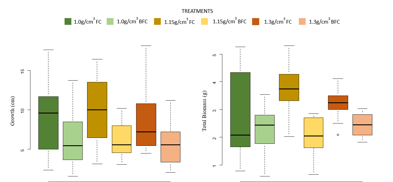
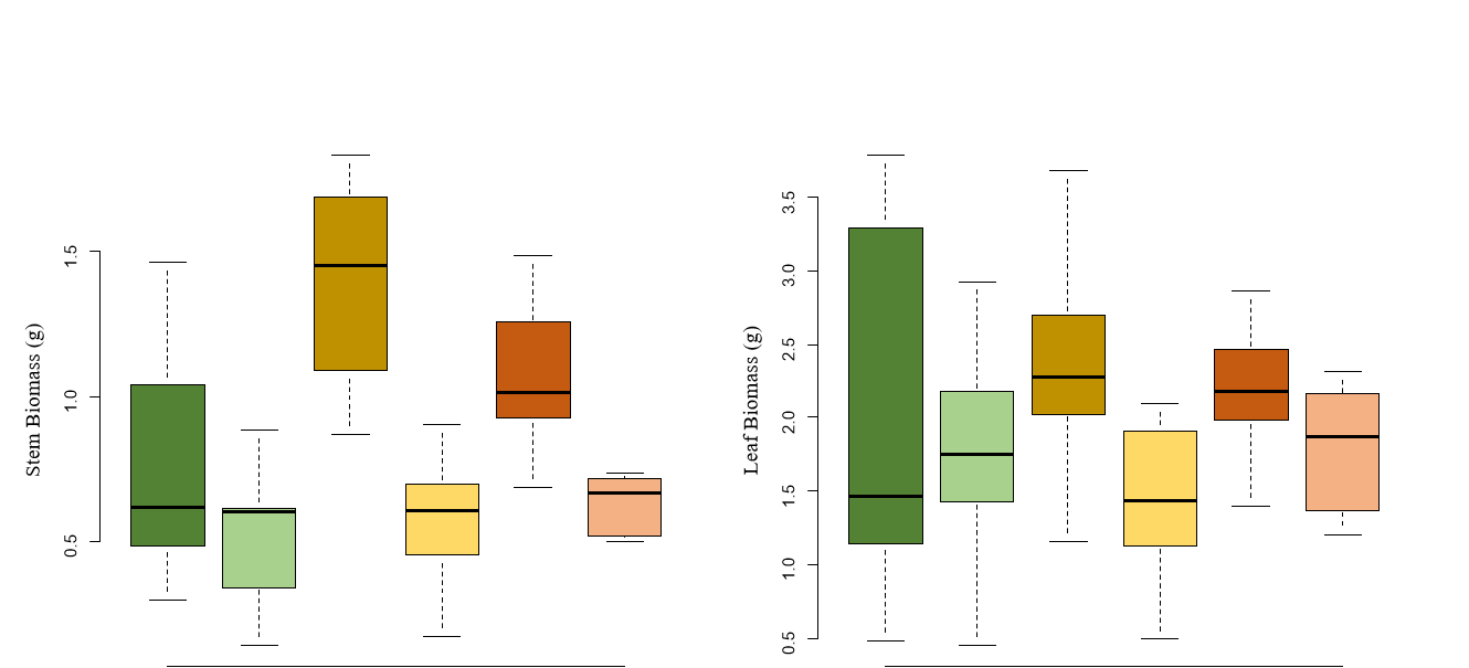
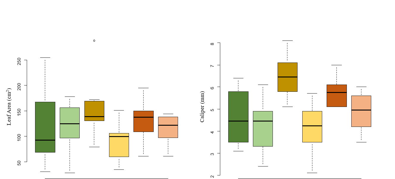
Figure 5. Box and whisker plots of (top left-bottom right): growth (cm)- measured from initial height of planting to final height at harvest; total biomass (g)- combined leaf and stem biomass (g); stem biomass (g); leaf biomass (g); leaf area (cm2); caliper(mm).
Interpretation
The above box and whisker plots represent the treatments used on the x-axis and the above ground measurements on the y-axis. The use of these graphs was to see the maximum and minimum measurements from each replicate. It also is used to determine if there are any skews, outliers, and to visualize the variation between each treatment. In Figure 5. we can see that most of the data is normally distributed. I can also see that the lower water potentials have less growth than the treatments at field capacity. For leaf area I can see that most of the data except for 1.3 at field capacity is skewed and shows no difference amongst treatments. While Caliper is mostly normally distributed with the opposite for skewness from leaf area coming from 1.3 at field capacity. I can also see that the treatment of 1.15 at field capacity has the greatest caliper. Which makes sense when looking at the stem biomass. The leaf biomass has the highest variation seen with 1.0 at field capacity, which most likely lead to the high variation in overall biomass. With treatment 1.15 at field capacity having the greatest overall biomass. Overall, the preliminary data exploration of the green house experiment showed that water potential influences plant growth and biomass.
The above box and whisker plots represent the treatments used on the x-axis and the above ground measurements on the y-axis. The use of these graphs was to see the maximum and minimum measurements from each replicate. It also is used to determine if there are any skews, outliers, and to visualize the variation between each treatment. In Figure 5. we can see that most of the data is normally distributed. I can also see that the lower water potentials have less growth than the treatments at field capacity. For leaf area I can see that most of the data except for 1.3 at field capacity is skewed and shows no difference amongst treatments. While Caliper is mostly normally distributed with the opposite for skewness from leaf area coming from 1.3 at field capacity. I can also see that the treatment of 1.15 at field capacity has the greatest caliper. Which makes sense when looking at the stem biomass. The leaf biomass has the highest variation seen with 1.0 at field capacity, which most likely lead to the high variation in overall biomass. With treatment 1.15 at field capacity having the greatest overall biomass. Overall, the preliminary data exploration of the green house experiment showed that water potential influences plant growth and biomass.
